Handling data displays for both new and seasoned editors can sometimes be tricky. There are standards or expectations for certain figure types. While not all editors are responsible for, or have the ability to, substantially edit figures and tables, most editors can make suggestions or pose queries to help ensure that data displays are accurate, complete, and clear. Herein is a brief primer on one of the most common figure types in the medical literature, including a short checklist that might be useful before acceptance, during figure creation, or incorporated into a journal’s instructions for authors.

We’ve all seen the figures—the 2 (or more) lines snaking upward (or downward) across a plot, called Kaplan-Meier or survival curves. So, why are they called “survival” curves? In this context, survival could be literal (mortality in study participants over the course of treatment) or it could mean the occurrence of a particular outcome over time, but not necessarily death (e.g., disease recurrence, a particular symptom). The main goal of this type of data display is to show differences in survival/event occurrence between groups (e.g., between those assigned to a new agent vs. placebo in a clinical trial).¹

Survival curves are often used in reporting major outcomes in studies; they are big-picture data displays. These plots are good for showing overall change over time, but not specific differences at discrete points.²

The curves themselves aren’t smooth as the term implies; they are a series of horizontal steps. In fact, some journals provide guidance to authors that the curves should be produced using a step function (not smoothed) when output from the statistical software program.

In these figures the outcome of interest is represented on the y-axis, and time is represented on the x-axis. The axis scales should be slightly larger than the range of values being plotted, so that the data are fully contained in the plot and take up most of the area.³

One thing authors and editors need to consider is the directionality of the curves: should the lines go up or down? A survival plot going down displays the proportion of patients free of the event (which of course declines over time), whereas a plot going up shows the cumulative proportion experiencing the event over time. In principle, both contain the same information, but the visual perceptions can be quite different.⁴

When the outcome of interest is relatively frequent (e.g., occurs in approximately ≥70% of the study population), event-free survival may be plotted on the y-axis from 0 to 1.0 (or 0% to 100%), with the curve starting at 1.0 (100%), i.e., at the top. When the outcome is relatively infrequent (e.g., occurs in <30% of the study population), it may be preferable to plot upward starting at 0 so that the curves can be continuous without breaking the y-axis scale, or so that the y-axis can be truncated before 100.⁵ Some might argue that the full scale (0–100) should always be included, but this may impair the ability to discriminate between treatments,³ especially if there are few events (which would crowd the curves at the top of the plot).

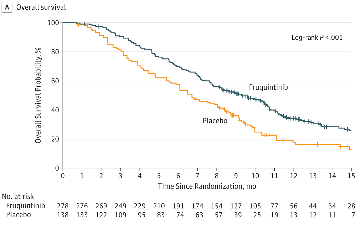
Some figures include placement of small vertical ticks on the curves to mark when individuals have had data censored due to withdrawal from the study, loss to follow-up, or remaining alive without event occurrence at last follow-up. If possible, label the curves directly instead of using a key, which enables readers to more quickly identify which line reports data for which group.

The extent of follow-up should be explained—e.g., by listing at regular intervals under the x-axis the number still in the analysis in each treatment group (i.e., “No. at risk”). Time-to-event estimates become less certain as the number of individuals diminishes, so consider ending the plot when a predetermined proportion is still in follow-up (e.g., 20% or 10%).⁵ Also, the mean or median length of follow-up for each group should be provided, either in the plot itself or in a figure legend.

Plots should include some indication of statistical uncertainty, such as error bars on the curves at regular time points, shading of 95% CIs, or an overall estimate of treatment difference, such as a relative risk or hazard ratio (with 95% CI) and/or log-rank P value. This information can be placed within the graph and/or in the legend.⁵

The example Figure herein illustrates the main components and requirements of a survival curve, and the checklist offers some guidance when building, editing, or reviewing these figures.

References and Links

1. Sullivan L. Survival analysis. [accessed May 17, 2021]. http://sphweb.bumc.bu.edu/otlt/MPH-Modules/BS/BS704_Survival/
2. Schriger DL, Cooper RJ. Achieving graphical excellence: suggestions and methods for creating high-quality visual displays of experimental data. Ann Emerg Med. 2001;37:75–87. https://doi.org/10.1067/mem.2001.111570
3. Graphs, charts, and parts of a graph. In: Council of Science Editors, Style Manual Committee. Scientific style and format. 8th ed. Chicago, IL: University of Chicago Press; 2014.
4. Pocock SJ, Clayton TC, Altman DG. Survival plots of time-to-event outcomes in clinical trials: good practice and pitfalls. Lancet. 2002;359(9318):1686–1689. https://doi.org/10.1016/S0140-6736(02)08594-X
5. Christiansen S, Manno C. Survival plots. In: Christiansen S, Iverson C, Flanagin A, et al. AMA manual of style: a guide for authors and editors. 11th ed. Oxford, UK: Oxford University Press; 2020. [accessed May 18, 2021]. https://www.amamanualofstyle.com/view/10.1093/jama/9780190246556.001.0001/med-9780190246556-chapter-4-div2-140
6. Li J, Qin S, Xu R, et al. Effect of fruquintinib vs placebo on overall survival in patients with previously treated metastatic colorectal cancer: the FRESCO randomized clinical trial. JAMA. 2018;319:2486–2496. https://doi.org/10.1001/jama.2018.7855

Stacy L Christiansen is Managing Editor, JAMA, and Chair, AMA Manual of Style committee.

Opinions expressed are those of the authors and do not necessarily reflect the opinions or policies of their employers, the Council of Science Editors, or the Editorial Board of Science Editor.